The history of deep learning
How is ChatGPT able to generate text? How can AI programs create images? The technology behind this is called deep learning.
A guest article by Jan Ebert Software Engineer and Researcher for Large Scale HPC Machines and Deep Learning, Forschungszentrum Jülich
The current revolution in artificial intelligence (AI) is being driven primarily by deep learning and large language models (LLMs). Delving deeper into the background is essential because knowledge is the best way forward. Only with the necessary knowledge can we understand the current situation and future developments. But how does deep learning work in the first place? In essence: it's mathmatics. This article provides an introduction to the most important technical principles of deep learning, neural networks and more.
What is deep learning?
The combination of
- a large number of tunable controls,
- a function with certain mathematical properties
- a lot of data to learn from (at least 10,000 examples)
- some form of comparison function/error measure, and
- a gradient-descent-based optimisation algorithm (explanation coming soon),
results in a very flexible algorithm that can solve all kinds of problems (including predicting human language!).
The technology behind deep learning is called a neural network.
When you strip away the magic, neural networks are just numbers that we add, multiply and apply some elementary mathematical functions to. Their amazing expressiveness comes from the way this mathematics between many numbers can capture even very abstract concepts.
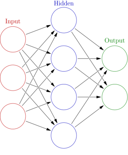
This diagram here shows a neural network with several layers.
- The input layer processes the data in a neural network.
- The output layer processes all its input values into a specified output format.
- Any other layer is called the hidden layer. In this case we have a neural network with a single hidden layer.
Each circle is a neuron, and the arrows between them represent the strength of the connection between these neurons, just like we humans have synapses that change their strength! You can see that different input neurons connect and send information to the hidden layer neurons, which in turn connect and send information to the output neurons.
In neural network jargon you will often come across the term "weight". A weight is the strength of an artificial synapse. The "model weights" are all the synaptic strengths across all the layers that make up the model.
Almost all modern neural networks are “differentiable”, which means that we can take their derivatives. A derivative represents the direction your curve moves towards when you slightly change the input (the x in f(x)). This is the key mathematical property that we need our model to fulfil so that we can use the currently popular ways of making our models learn.
There is one more ingredient to add, the comparison function we mentioned before. To improve something, we need to know whether we actually get better or worse. For very simple questions, we can for example measure if we answered yes or no correctly. Or when we do math, we can measure how far away we are from the correct result. We want to minimize the amount of error that we measure with this comparison function. And for that to be possible, we again need differentiability.
For now, try to ignore which function we are actually trying to optimise. Stochastic gradient descent is an optimisation algorithm that works like this:
- First you take the derivative of the function you want to optimise. This is very similar to what you might have done at school; in deep learning we just do it for many x at once. To train LLMs, we do it for extraordinarily many x at once.
- Follow the derivation in the opposite direction, taking an "optimisation step". Intuitively, this means that we try to evaluate our function closer to its optimal point. We move x so that hopefully f(x) becomes "better", more like what we want it to be. For an LLM, this would mean that we move all of its parameters a little bit in the hope that it will become better at predicting successive texts.
- Go back to step 1 until you're happy with the result.
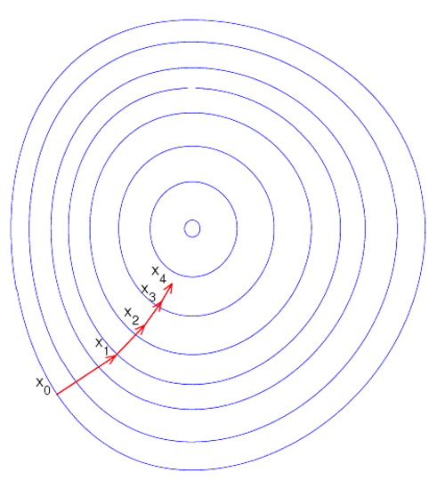
This diagram above shows the four steps of a very well-working gradient descent optimization. We immediately find our way to the optimum at the smallest circle in our function landscape. While in practice, it’s sadly not so easy, we will not concern ourselves with such pessimism today.
Where does the name come from? The derivative for many inputs is also called a gradient, and the optimization steps descend towards the minimum of the measured error.
Connectionist history
Surprisingly, the basic methodology we use today was established very early and has been very stable ever since.
In the 1950s, the first wave of research on artificial neural networks began with the first mathematical formalisations of neuron-based learning methods. With the invention of the backpropagation algorithm, one of the most fundamental methods of deep learning, in 1970, and the increasing speed and availability of computers, the second wave began in the 1980s. It was during this period that the neural network architectures still in use today began to produce impressive practical results.
For example, the Neocognitron, a vision model, was used to recognise handwritten Japanese characters. In 1997, the Long Short-Term Memory (LSTM) model was published, a sequential model that could solve problems requiring knowledge of the past. It is important to emphasise that these models were self-learning; the performance was not manually programmed into the models. Instead, the models saw examples and learned from them.
The LSTM is of particular interest to us because for 20 years it was the language model of choice, producing the most impressive results. Although it was also used for other tasks in natural language processing (speech-to-text, stock market predictions, drug design, playing extremely complex video games, ...), its most practical successes were achieved in natural language processing. Soon, every phone was using LSTMs to predict the next word you were going to type or to recognise speech.
In the third wave, starting in the late 2000s, advances in computer hardware and the amount of readily available data finally revolutionised deep learning, making it the important and mainstream field it is today. LSTMs and vision models began to win competitions in research challenges, beating all previous methods based on decades of manual development, and making people aware of the power of deep learning and artificial intelligence.
We leave you with a brief conclusion to the historical journey. The basis for LSTMs, called recurrent neural networks (RNNs), was invented as early as 1920 and 1925 with the Ising model. The Ising model could not learn, it was static, and it was not until 1972 that the first learning RNN was developed. This was then improved to become the LSTM in 1997.
Today, in 2024, we can look back and see how far the field of deep learning has come in the last 100 years, becoming the backbone of one of the most important paradigm shifts we are currently experiencing.
Learn more
If you are interested in the topic and would like to know more about deep learning and its various applications: Jan Ebert gave a presentation as part of our "HIDA Lecture Series on AI and LLMs", which we have recorded.
Watch the recording (YouTube video)
You can also download the presented slides with all information here: